Distribution Analysis of Feature Map and Gradients in Mobilenet and Resnet Model Layers using Glorot and He`s initialization
Copyright ⓒ 2021 The Digital Contents Society
This is an Open Access article distributed under the terms of the Creative Commons Attribution Non-CommercialLicense(http://creativecommons.org/licenses/by-nc/3.0/) which permits unrestricted non-commercial use, distribution, and reproduction in any medium, provided the original work is properly cited.

Abstract
Initializing the weights plays an essential role in a convolutional neural network model. This paper investigates how Glorot and He's initialization methods behave in Mobilenet and Resnet models on the weeds classification problem. Experiments show that pointwise and depthwise convolution in Mobilenet reduces the variance of feature maps from earlier layers. Using the He’s method, shortcut connection in Resnet saturate values in logistic classify layer. The accuracy of Mobilenet and Resnet, using Glorot's method, are 0.9568 and 0.9711, respectively. While using He's method, we obtain 0.9471 using Mobilenet and 0.9645 using Resnet. Also, both models converge faster and better generalization using Glorot's method than using He's method.
초록
합성곱 신경망 모델에서 가중치를 초기화하는 것은 모델 성능 향상에 필수적인 역할을 한다. 본 논문은 Mobilenet 및 Resnet 기반 잡초 분류를 위한 합성곱 신경망 모델에 Glorot 및 He 초기화 방법을 분석한다. 본 실험 결과 Mobilenet의 Pointwise와 Depthwise 컨벌루션이 초기 레이어의 특징 맵의 변화를 줄이고, Resnet의 단축경로 연결은 He 초기화를 사용할 때 로지스틱 분류 레이어에서의 값을 포화시킨다. Glorot 초기화 방법을 사용한 Mobilenet 및 Resnet 기반 잡초 분류 합성곱 신경망 모델의 정확도는 각각 0.9568과 0.9711이고, He 초기화 방법을 사용한 경우에는 각각 0.9568과 0.9711이다. 따라서 Glorot 초기화 방법을 사용할 경우 He 초기화 방법보다 합성곱 신경망 모델이 더 빠르게 학습되고 일반화에 좋다.
Keywords:
Weights initialization, Glorot initialization, He initialization, Convolutional neural network, Weeds classification키워드:
가중치 초기화, Glorot 초기화, He 초기화, 컨볼루션 신경망 네트워크, 잡초 분류Ⅰ. INTRODUCTION
Many researchers have used convolutional neural network (CNN) models and achieved state-of-the-art performances in many computer vision problems, such as object detection, classification, and retrieval. These models are either trained from scratch or used transfer learning to initialize weights in models. Transfer learning applies weights trained from a source domain as initial parameters to a target domain. In practice, many deep learning frameworks such as Tensorflow [1], Keras [2], or PyTorch [3] support CNN models trained on the ImageNet dataset for transfer learning purposes. As shown in [4], we can apply transfer learning to guide the model to converge quickly, as long as the information features in the target domain are similar to those in the source domain. Otherwise, training the model from scratch is a reasonable solution. But this type of training requires careful initialization of learnable weights so that the model can learn features efficiently.
From a classical shallow LeNet-5 model to the deep VGG, Mobilenet, and Resnet CNN models, in general, a CNN model architecture consists of many “stacks” convolutional layers, where the output feature maps of a layer are the input of other layers. A matrix multiplication operates the convolution operators between the feature map and filter (followed by an activation function, such as sigmoid or rectified linear unit (ReLU)). The distribution of learnable parameters in filters affects the distribution of values in the output feature maps. Therefore, large weights tend to saturate feature maps towards 0 and 1 using sigmoid or lead to computational overflow using ReLU. Conversely, small weights may make the distribution of feature maps tight around zero in deeper layers, leading to small gradients and harmful model performance.
Probabilistic analysis of initialization of weights has been studied to avoid saturation or small gradient problems. LeCun et al. [5] showed that initializing the weights by randomly drawn from a zero-mean distribution makes the distribution of output nodes in the artificial neural network (ANN) model approximate a standard deviation of 1. This unit standard deviation places the node value in the linear curve of the sigmoid function so that the model can converge efficiently. However, the sigmoid function reduces the model’s ability to learn features (due to its non-zero mean) and may induce important singular values in the Hessian matrix. Glorot and Yoshua [6] clarified this phenomenon by experimenting with a multi-layer perceptron with a sigmoid activation function. They found that the sigmoid activation values in all layers are saturated to 0. To solve this problem, they studied and proposed a probabilistic approach to initialized weights so that variances of these weights were similar across layers (we call it Glorot's method). This method helps the gradients propagate with similar variance from lower to upper layers so that the model may learn features efficiently. But their approach is based on symmetric activation functions such as sigmoid, hyperbolic tangent, and softsign, which may be unsuitable for ReLU. He et al. [7] followed the ideas of Glorot and Yoshua [6] but examined the rectifier nonlinearities functions such as ReLU. They proposed a weights initialization method that works for nonlinear rectifiers (He's method). Given a Resnet model with ReLU as the activation function, Glorot's method makes the model stall, especially on extremely deep models. In contrast, He's initialization can make the model well converged.
In this paper, we investigate and compare the quality of Glorot and He's methods on Mobilenet and Resnet models. We show weight distributions, feature map values, and backpropagation gradients in both models on the CNU weeds dataset. By visualizing the feature map distribution, we realize that pointwise and depthwise convolution in Mobilenet reduces the variance of feature maps in deeper layers. Using the He's method, the shortcut connection in Resnet causes the last layer to saturate, and both models converge slower and generalize worse than using the Glorot's method. In experiments, Mobilenet and Resnet have an accuracy of 0.9568 and 0.9711 using Glorot's method; and 0.9471 and 0.9645 using He's method.
Ⅱ. CNU WEEDS DATASET
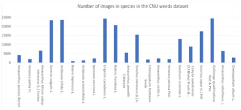
We used the CNU weeds dataset for experiments. This dataset was constructed by the Department of Electronics and Computer Eng, CNU, Gwangju, under the supervision of Rural Development Administration, Republic of Korea. Weeds images were captured and collected by Korean plant taxonomists, whose majors are botany. They collected weeds images on farms, fields in the Republic of Korea by using high-definition resolution cameras. Those species were classified and grouped by the international standard of plant taxonomy. This dataset has 21 species; it has 208,477 images in total. As shown in Figure 2, the CNU weeds dataset is an imbalanced dataset, where the species that has the largest number of images is Galinsoga quadriradiata Ruiz & Pav., around 24300 images. In contrast, species Bidens bipinnata L. has the smallest number of images, about 800 images.
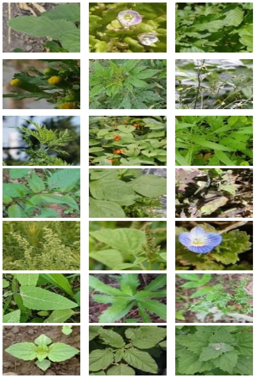
Figure 1 shows an example of images on the CNU weeds dataset. From an agricultural perspective, weeds belonging to a particular family share some common characteristics in their structure, making their morphology quite similar even though they belong to two different species. On the other hand, weeds of different species are entirely different in appearance.
Ⅲ. CNNs
3-1 Mobilenet
Howard et al. [8] developed a CNN model capable of deploying in low-memory devices called Mobilenet. This model has two core layers: Depthwise and pointwise convolution.
In standard convolution, current feature maps are formed by a multiplication and summation between previous feature maps and current filters. However, many filters lead to a huge number of learnable weights. To reduce the number of weights, Mobilenet split this convolution into two types of convolutions: First, a depthwise convolution applies a single convolutional filter for each channel in the feature maps. Mathematically, we can formulate depthwise convolution as
| (1) |
where is the depthwise convolutional filter of size Dk × Dk × M. The mth filter in is applied to the mth channel in F.
Then, a pointwise convolution (or 1 × 1 convolution) is applied to aggregate information in the feature maps channel-wise. A 3 × 3 depthwise convolutional filter in Mobilenet reduces 8 to 9 times computation than standard convolution.
In experiment, Howard et al. [8] showed that Mobilenet got a high accuracy on fine-grained object classification. So Mobilenet is sufficient for the weeds classification problem.
3-2 Resnet
Typically, CNN architecture models have “stacked” layers: One layer is placed on top of each layer. This type of deep architecture results in vanishing or exploding gradient flows from the bottom to the top layers, thus preventing the model from converging. He et al. [9] presented a residual learning framework to conveniently train an extremely deep model. Mathematically, a building block of the Resnet model is formulated as
| (2) |
where x and y are the input and output feature maps of residual block, F is the residual mapping. In practice, this function is a stack of convolutional layers, each layers contain filters, and each i-th filter has a weights matrix Wi. The summation operation is performed by an element-wise addition of the input feature maps x to the stacked layers and the output feature maps of these stacked layers.
Resnet contains many building blocks. As explained in [10], implementing Eq. (2) recursively, we have
| (3) |
| (4) |
| (5) |
for any shallow layer l. Assign Eq. (5) as xL and denote the loss function as ϵ, the gradient of ϵ with respect to the feature map xL is
| (6) |
| (7) |
δϵ/δxL is unlikely to be zero, so the gradient does not get vanish. With this building blocks, Resnet contains many deep layers and avoid making the gradient vanish or explode.
Ⅳ. WEIGHT INITIALIZATION
4-1 Glorot
Glorot and Bengio [6] analyzed layers in an ANN model by estimating the distribution of activation values (output of symmetry, nonlinear activation function) and gradients. They initialized weights followed by a random distribution and used the standard stochastic gradient descent (SGD) to optimize weighs in this model. They found that weights distribution in deeper layers saturate toward 0. With the sigmoid activation function, this behavior prevents the gradients from flowing backward so that deeper layers may not learn valuable features. This phenomenon also occurs for softsign and hyperbolic tangent but is less extreme for sigmoid. In common, SGD from random initialization is inefficient for a deep neural network.
To keep the information flow from saturating, they proposed a new initialization method to preserve the variance of output activation values between layers.
| (8) |
where zi,zi' is the activation outputs of layer i and i' respectively. Finally Eq. (8) led to
| (9) |
where x was the network input.
Assume we use a symmetry, zero-centered activation function with unit derivative at 0. Using 1st order Taylor function, we can approximate as a linear function as Eq. (10)
| (10) |
In common, at layer i, ANN models calculate a linear combination si between weights Wi and output of the activation function zi, and the bias term bi is added. That is, si = ziWi+bi, and zi+1f(si). Assume weights are initialized independently. To obtain similar variance, we calculate
| (11) |
| (12) |
| (13) |
Initializing the bias term as zero lead to Var[bi-1] = 0, we have
| (14) |
| (15) |
| (16) |
| (17) |
where is the number of nodes in layer. Assume we initialize weights by using a zero-mean distribution function, then
| (18) |
| (19) |
Eq. (19) is a recursive formular. Expanding to all layers, we have
| (20) |
Setting ni' Var[Wi'] = 1 satisfy Eq. (8).
We also want similar gradient variance across layers, means that
| (21) |
where is a cost function of the ANN model. Using chain rule, we have
| (22) |
| (23) |
| (24) |
Eq. (24) is also having a recursive form. Expanding to all layers, we have
| (25) |
Setting ni'+1 Var[Wi'] = 1 satisfy Eq. (21). In total, for all, we have the following system of equation.
| (26) |
| (27) |
Eq. (27) show that the variance of weights in layer i depend on the number of nodes in that layer and the next layer. Assume we initialize weights followed by a uniform distribution, Wi ~ U(-a,a), then
| (28) |
4-2 He
Glorot's method is based on the assumption of using a zero-centered symmetric function as the activation function. However, this function is unsuitable for deep neural networks because of the gradient vanish problem during backpropagation [5]. Many popular CNN models such as VGG [11], Resnet [9], Mobilenet [8] used rectifier nonlinear activation functions because this function accelerates the training convergence [12] and more generalizes the model than symmetry function [13]. He et al. [7] investigated the variance condition of the output of rectifier nonlinear activation function at layer in a stacked CNN model, based on the procedure of Glorot’s method.
| (29) |
where x is k2c × 1 vector, c is the number of channels and k is the filter size. W is a d × n weight matrix containing d filters, n is k2c is the number of connections. Because we stack layers, the number of channels in current layer are equal to the number of filters used in the previous layer, cl = dl-1.
At the beginning, we set the bias term bl = 0 and xl = f(yl-1). Assume we initialize weights Wl followed by a zero-mean distribution (E(Wl) = 0), then
| (30) |
| (31) |
| (32) |
| (33) |
| (34) |
Using rectified linear unit function, we have x = f(y) = max(0,y), so
| (35) |
| (36) |
| (37) |
Since y2 is a symmetric function around 0 and the input y is zero-mean, we have
| (38) |
| (39) |
| (40) |
| (41) |
So we have
| (42) |
| (43) |
Expand recursive Eq. (43) to all L layers, we have
| (44) |
Similar to Glorot’s method, He’s method maintains variance in the activation output across all layers by setting a condition for all layers,
| (45) |
Denote Δx = δϵ/δx, Δy = δϵ/δy, where Δx is a c × 1vector, represents gradient at a pixel of this layer, Δy represents k × k pixels in d channelks, and ϵ is an objective function. We have
| (46) |
| (47) |
where is a matrix, and . Assume that Wl is initialized by a symmetric distribution around zero, then E[Δxl] for all l. By using ReLU as the activation function, f'(yl) = 1 or 0 with equal probability, so
| (48) |
| (49) |
| (50) |
So, calculate variance in Eq. (47), we have
| (51) |
| (52) |
Put L layers together, we have
| (53) |
To maintain gradient variance in backpropagation, we set for all layers l. He et al. [7] stated that using either nl or were sufficient for training the model. This condition aims to keep the gradient from being exponentially large or small.
He’s method show that the weights in layer are initialized with a variance that depend only on the filter size in that layer. If we initialize Wl~U(-a,a), then
| (54) |
Mathematically, a filter of size nl applied to layer l has a larger variance using He`s method than that of Glorot. By considering Eq. (28) and Eq. (54), Glorot requires an additional filter of size nl+1 in the next layer l+1, which increases the denominator value, hence smaller variance than He.
Ⅴ. EXPERIMENTS
We used the CNU weeds dataset to train Mobilenet (88 layers) and Resnet model (50 layers). We trained on 100 epochs, using SGD with Nesterov momentum to optimize the cross-entropy loss function. The learning rate was initialized as , and decay to and at the 30th and 60th epoch. The batch size was 128 for Mobilenet and 32 for Resnet. We finetuned the model by adding a 256 dimension fully connected layer to avoid overfitting problems, followed by a batch normalization layer and ReLU activation function. We set the size of input color images to and normalized to using Mobilenet, and per-pixel mean subtraction using Resnet, as applied in [8] and [9].
We divided 60% of images in each species on the CNU Weeds dataset as training set, 20% as validation set, and the remaining 20% as test set. During model training, we selected the weights that had the highest accuracy on the validation set.
5-1 Weight Initialization
We initialized weights using a zero-mean Uniform distribution with variance followed by Glorot and He's methods. Figures (a) and (b) in Figure 3 show the box plot of values in filters, output of activation layers, and gradients between layers. It turns out that these values, using He's method, had a higher variance than Glorot‘s method because mathematically, He's method only needs the filter size in the current layer, while Glorot's method requires the current and next layer. Both Mobilenet and Resnet have large filter sizes at deeper layers, thus reducing its variance then. In particular, variances of the output of activation layers in Mobilenet decreased faster than those in Resnet, starting from the depthwise and pointwise convolution layers. The large filter size configuration caused this issue in the earlier layers in Mobilenet.
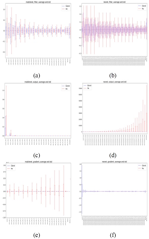
Box plot of values in filters, output of activation layers, and gradients across layers, using Glorot and He’s methods. Left column: Mobilenet. Right column: Resnet
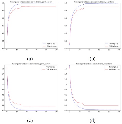
Training and validation curve on Mobilenet. (a) Accuracy, Glorot. (b) Accuracy, He. (c) Loss, Glorot. (d) Loss, He.
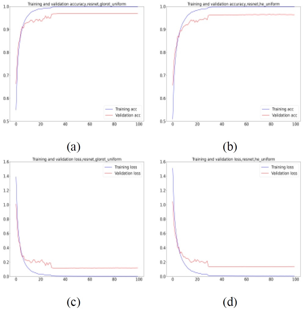
Training and validation curve on Resnet. (a) Accuracy, Glorot. (b) Accuracy, He. (c) Loss, Glorot. (d) Loss, He.
The first two rows of Figure 6 show the Mobilenet output activation values distribution, using Glorot and He's methods. The first layer in this model is a standard convolution. The left-most figures in 2 rows show that the output of this layer had a higher variance using He’s method than Glorot’s method. The last two figures of Figure 6 and figure (c) in Figure 3 show that, on average, using both initialization methods brought weights approaching zero. Both methods had a small variance when we went to deeper layers, mainly affected by two reasons: small input values after normalization ([-1,1]) and small variance of the zero-mean depthwise and pointwise convolution layers.
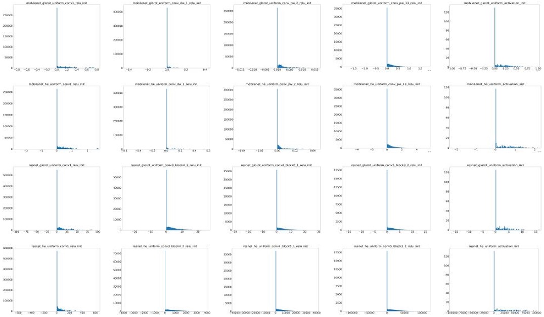
Distribution of output of activation function. From top to down, 1st and 2nd row use Glorot and He on Mobilenet, 3rd and 4th row use Glorot and He on Resnet. From left to right is the result from earliest to lowest layers.
The last two rows of Figure 6 show the distribution of Resnet output activations. Like Mobilenet using Glorot's method, the variance decreased as we went to deeper layers, as shown in figure (d) of Figure 3. In contrast, using He's method increased the variance rapidly. In the last layer, many weights are larger than 105, resulting in the maximum value of softmax activation function saturated to 1. Thus, the gradient of all weights (after applying chain rule) was approximate zero. Those large weight values in deeper layers came from 2 reasons: For one layer, the distribution variance using He's method is larger than using Glorot‘s method, and the skip connection by a summation in Resnet architecture increases the output values in deeper layers.
The distribution of gradients in Mobilenet is shown in the first two rows in Figure 7, using Glorot and He’s methods. Figure (e) in Figure 3 in both methods shows a lower variance in gradient in deeper layers for Glorot‘s method. In contrast, gradients have large values in deep layers for He’s method, except for the values in pointwise convolution layers.
| (55) |
| (56) |
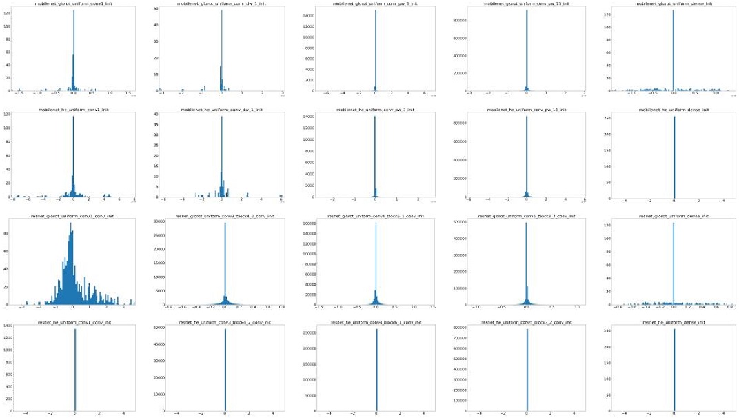
Distribution of output of gradient. From top to down, 1st and 2nd row use Glorot and He on Mobilenet, 3rd and 4th row use Glorot and He on Resnet. From left to right is the result from earliest to lowest layers.
The last two rows in Figure 7 show the distributions of gradient values in the Resnet model, using Glorot and He's methods. It shows that using Glorot‘s method, many weights had non-zero gradients. Except for the first layer, all layers had similar output variance, as shown in figure (f) of Figure 3. Using He's method to initialize weights in the Resnet model, all the gradients across layers were very close to zero. As explained above, large variance in He's method and shortcut connection led to enormous value in deeper layers. Therefore, max(s) in Eq. (55) (softmax function, K is the number of classes) was approximately 1, and other elements in the softmax output vector were close to 0. In this case, the partial derivative in Eq. (56), where δij is the Kronecker delta function, was approximately zero with respect to any zj.
5-2 Performances
Figure 4 shows performances of training the Mobilenet, where the weights were initialized using the Glorot and He's methods. It indicates that Glorot‘s method helped the model to converge faster than using He. By using Glorot's method, the model increased in accuracy quickly, faster than He‘s method. In both methods, the model converged at the 30th epoch.
Figure 5 shows performances of training the Resnet. Like what was in Mobilenet, Glorot‘s method helped the model converge a bit faster, starting in the 10th epoch. The model converged at 30th epoch in both methods.
Table 1 shows performances of models using Glorot and He’s methods as initialization methods. In particular, Glorot‘s method showed the ability to generalize the model better than He‘s method when all metrics using Glorot‘s method were 0.01 points higher than He‘s method, except for the loss value showing that Glorot‘s method was lower than He‘s method by nearly 0.03 points. Besides, Resnet had higher performance than Mobilenet, regardless of the initialization method used.
5-3 Analysis
Experiences have shown that, for a model, using Glorot's method to initialize weights makes the model converge faster and more general than He's method. The first few epochs in Figure 4 and Figure 5 indicate that, for the CNU weeds dataset, Glorot's method to initialize the weights placed these weights in appropriate positions on the loss surface in both models. This result is in contrast to [9], where Glorot's method (based on symmetric activation functions) is more suitable for training a weeds classification model than using He's method (based on rectifier nonlinear activation functions). Remind that both models use ReLU as the activation function. This problem occurs when the architectures of both models are not deep enough to show the advantage of He‘s method over Glorot‘s method.
Glorot and He's methods is founded based on the assumption of stacking standard convolution layers such as VGG or conventional ANN model. However, both model architectures have its characteristic that may not fit that assumption. As shown in Figure 6, pointwise and depthwise convolution in Mobilenet reduces the variance of the output of activation function, resulting in the output in deeper layers close to zero. Shortcut connection in Resnet enlarged variance when using He's method, but not in Glorot’s method because the variance in Glorot’s method is smaller than He’s method. This means that we might deal with large weights initialization, resulting in saturation in Glorot’s method is smaller than He’s method.
Ⅵ. CONCLUSION
In this paper, we compared and analyzed the performance of CNN models in the CNU Weeds dataset for weeds classification. We trained the Mobilenet and Resnet models from scratch, using Glorot and He's methods to initialize the weights. These authors studied these methods in conventional ANN and CNN models to maintain the variance of output of activation function across layers. But in practice, specific layers in Resnet and Mobilenet made these methods behave unexpectedly. Pointwise and depthwise layers in Mobilenet reduced the variance to near zero, and shortcut connection in He’s method expanded the variance in deeper layers leading to saturation in softmax layer. Experiments show that using Glorot's method placed weights in both models in convenient positions so that models converged more quickly and generally than using He's method.
Acknowledgments
This work was carried out with the support of "Cooperative Research Program for Agriculture Science and Technology Development (Project No. PJ01385501)" Rural Development Administration, Republic of Korea.
References
- TensorFlow, “Transfer learning and fine-tuning,” TensorFlow, 17 06 2021. [Online]. Available: https://www.tensorflow.org/tutorials/images/transferlearning, .
- F. Chollet, “Transfer learning & fine-tuning,” Keras, 12 05 2020. [Online]. Available: https://keras.io/guides/transfer_learning/#transfer-learning-amp-finetuning, .
- S. Chilamkurthy, “TRANSFER LEARNING FOR COMPUTER VISION TUTORIAL,” Pytorch, [Online]. Available: https://pytorch.org/tutorials/beginner/transferlearningtutorial.html, .
- B. Neyshabur, H. Sedghi and C. Zhang, “What is being transferred in transfer learning?,” Advances in Neural Information Processing Systems, vol. 33, pp. 512-523, 2020.
-
Y. LeCun, L. Bottou, G. B. Orr and K. R. Müller, “Efficient BackProp,” Neural Networks: Tricks of the Trade, pp. 9-50, 1998.
[https://doi.org/10.1007/3-540-49430-8_2]

- X. Glorot and Y. Bengio, “Understanding the difficulty of training deep feedforward neural networks,” in Proceedings of the 13th international conference on artificial intelligence and statistics, 2010.
- K. He, X. Zhang, S. Ren and J. Sun, “Delving Deep into Rectifiers: Surpassing Human-Level Performance on ImageNet Classification,” in 2015 IEEE International Conference on Computer Vision (ICCV), 2015.
- A. G. Howard, M. Zhu, B. Chen, D. Kalenichenko, W. Wang, T. Wetand, ... and H. Adam, “Mobilenets: Efficient convolutional neural networks for mobile vision applications,” in arXiv preprint arXiv:1704.0486, , 2017.
- K. He, X. Zhang, S. Ren and J. Sun, “Deep residual learning for image recognition,” in Proceedings of the IEEE conference on computer vision and pattern recognition, 2016.
- K. He, X. Zhang, S. Ren and J. Sun, “Identity mappings in deep residual networks,” in European conference on computer vision, 2016.
- K. Simonyan and A. Zisserman, “Very Deep Convolutional Networks for large-Scale Image Recognition,” in 3rd International Conference on Learning Representations, San Diego, 2015.
- A. Krizhevsky, I. Sutskever and G. E. Hinton, “Imagenet classification with deep convolutional neural networs,” in Advances in neural information processing systems, 2012.
- X. Glorot, A. Bordes and Y. Bengio, “Deep sparse rectifier neural networks,” in Proceedings of the 14th international conference on artificial intelligence and statistics, 2011.

2017년 : Department of Mathematics, Computer Science, Ho Chi Minh University of Science (공학학사)
2020년 : 전남대학교 전자공학과 (공학석사)
2020년~현 재: 전남대학교 ICT융합시스템공학과 박사과정
※관심분야:디지털 신호처리(Digital signal processing), 영상 처리(Image processing), 머신러닝(Machine learning), 딥러닝(Deep learning) 등

2021년 : 전남대학교 전자공학과 (공학학사)
2021년~현 재: 전남대학교 ICT융합시스템공학과 석사과정
※관심분야:영상 처리(Image processing), 머신러닝(Machine learning), 딥러닝(Deep learning) 등

2018년 : 전남대학교 전자공학과 (공학석사)
2006년~현 재: Insectpedia 대표
2018년~현 재: 전남대학교 ICT융합시스템공학과 박사과정
※관심분야:디지털 신호처리(Digital signal processing), 영상 처리(Image processing), 머신러닝(Machine learning), 딥러닝(Deep learning) 등

1986년 : 서울대학교 전자공학과 (공학학사)
1988년 : 서울대학교 전자공학과 (공학석사)
1994년 : 서울대학교 전자공학과 (공학박사)
1995년~현 재: 전남대학교 ICT융합시스템공학과 교수
※관심분야:디지털 신호처리(Digital signal processing), 영상 처리(Image processing), 음성 신호처리(Audio signal processing), 머신러닝(Machine learning), 딥러닝(Deep learning) 등
