ChronoPatternNet: Revolutionizing Electricity Consumption Forecasting with Advanced Temporal Pattern Recognition and Efficient Computational Design

Ⅰ. Introduction

Electricity, as a vital element of modern life, necessitates robust and accurate forecasting methods to ensure efficiency and safety. With increasing dependency on electrical systems, the significance of predictive monitoring to prevent incidents and optimize usage has never been more paramount[1],[2]. Traditional forecasting methods, such as ARIMA[3] and Gaussian processes[4], have been foundational in this domain. However, these approaches often struggle with scalability and flexibility, especially in adapting to new data inputs, which is crucial in the dynamic landscape of electricity usage.

While foundational, these traditional models have notable limitations in handling the evolving complexity of electricity consumption data. ARIMA, a widely used method for time series forecasting, is constrained by its linear nature and assumption of stationarity, making it less effective in capturing nonlinear patterns and abrupt changes in electricity usage[5],[6]. Gaussian processes, offering a probabilistic approach, face challenges in scaling to large datasets and require extensive computation, limiting their practicality in realtime forecasting scenarios[7].

To deal with the complexity and larger data, deep learning-based methods were then introduced such as Recurrent Neural Networks (RNNs) with Long Short-Term Memory (LSTM) and Gated Recurrent Units (GRU), Convolutional Neural Networks (CNNs) with Temporal Convolutional Networks (TCN), and the more recent Transformer architectures[8]. Nevertheless, LSTM and GRU networks, while addressing some limitations of traditional models, encounter their own challenges. These include issues with gradient dynamics and insufficient memory retention[9]. Concurrently, TCN models, which represent a significant development in sequence modeling, however dilated convolutions in TCN, although useful for long-range dependency capture, can substantially raise computational and memory demands, particularly with lengthy or high-dimensional data[10]. The Transformer architecture, despite its proficiency in handling long sequences, grapples with demands of large datasets and computational intensity[11],[12], particularly in realtime forecasting – a critical aspect for electricity consumption monitoring.

To address these challenges, this paper introduces the "ChronoPatternNet" model, a novel approach to time series forecasting, with a focus on electricity consumption prediction. Contributions of ChronoPatternNet:

• Innovative pattern recognition: ChronoPatternNet introduces a novel method for identifying and leveraging repetitive patterns in electricity usage, enhancing the model's ability to make accurate forecasts based on historical data.

• Computational efficiency: By optimizing data processing through CNN architecture, our model achieves higher efficiency in both training and inference, making it viable for realtime forecasting and deployment on devices with limited resources.

• Adaptability to varied forecasting scenarios: Demonstrated effectiveness in both short-term and long-term forecasting scenarios, addressing a common limitation in existing models.

• Practical real world application: The compact and efficient design of ChronoPatternNet makes it a practical solution for real world energy forecasting, especially in smart grid systems.

• Open source contribution: With the public release of our model's source code, we aim to facilitate further research and development in the field, encouraging collaboration and innovation. The source code is available at https://github.com/andrewlee1807/ChronoPatternNet.

The remainder of this paper is structured as follows: Section 2 delves into related work, setting the stage for our contributions. Section 3 articulates the methodology behind ChronoPatternNet, followed by Section 4, which details our experimental evaluations on a comprehensive dataset. Section 5 discusses the implications and conclusions of our work.

Ⅱ. Related Work

The analysis of energy consumption involves leveraging time-series data for forecasting, employing classical statistical models, deep learning, and structured state-space models. Statistical methodologies, such as ARIMA models and clustering techniques, are widely used in electronic consumption forecasting[13]-[15]. Despite their effectiveness in specific scenarios, these traditional statistical models encounter challenges when dealing with complex, non-linear, and noisy datasets, emphasizing the need for advanced methodologies[16].

In the context of deep learning, approaches like Long Short Term Memory (LSTM) and Sequence to Sequence (S2S) models are explored for short-term load forecasting[17]-[20]. The DeepAR method introduces an autoregressive recurrent neural network designed for accurate probabilistic forecasts by training on a substantial dataset comprising interconnected time series[21].

Temporal Convolutional Networks (TCNs), including the proposed SCINet, emphasize the preservation of temporal relationships. SCINet introduces a lightweight model with a stride–dilation mechanism to address the heaviness of TCN models[10],[22],[23].

In the realm of Transformer based models, advancements like Informer, Autoformer, and Fedformer enhance time series forecasting[24]-[26]. However, recent research indicates that basic linear models, as exemplified by TiDE, can outperform certain Transformer based approaches in long-term time-series forecasting[27]. The announcement of TimeGPT-1[28] introduces a foundational model for time series forecasting, showcasing the effective application of insights from other AI domains to time series analysis.

Fig. 1.

Characteristics of electricity consumption-time series data

Recognizing the limitations of Transformers in handling real world time series data, the Structured State Space (S4) model emerges as a more efficient alternative, combining advantages from both CNNs and RNNs. This integration preserves interpretability while leveraging the power of deep learning to extract intricate patterns[29]-[31]. The emphasis on fusing global and local patterns for improved predictions remains crucial, given that recent deep learning models often remain one dimensional and demand high computational resources[32]. Hence, employing mixtures of repetitive temporal patterns remains a practical strategy to address long-dependency time series[17], as emphasized in this study.

Ⅲ. Methodology

This section provides a comprehensive overview of the Chronological Pattern Recognition Network (ChronoPatternNet), focusing on its approach to univariate, multi-step time series forecasting in the context of electricity consumption.

3-2 ChronoPatternNet Architecture

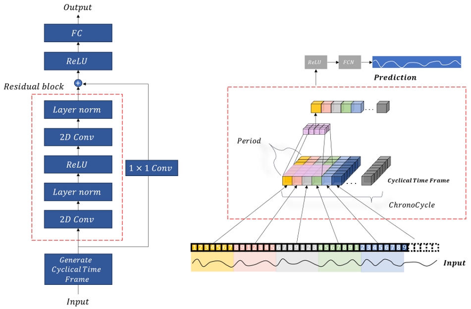
An overview of ChronoPatternNet architecture is illustrated in Fig. 2.

Fig. 2.

ChronoPatternNet's architecture

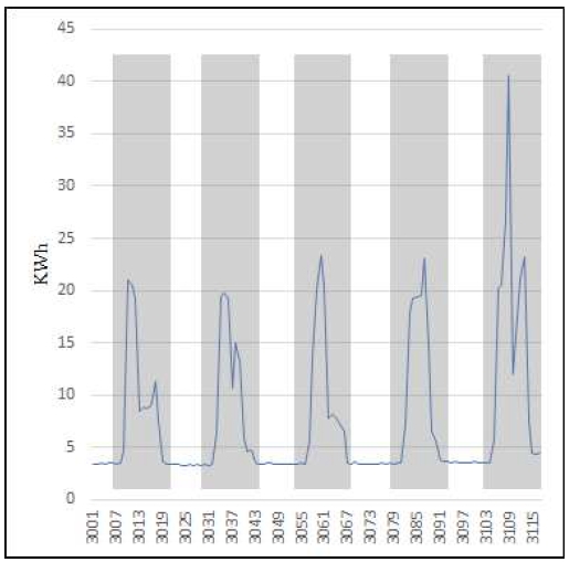
The core of ChronoPatternNet's architecture is grounded in the identification and analysis of recurrent patterns within time series data of electricity usage. As illustrated in Fig. 1, the time series is decomposed into segments, S_i = {s_i1,s_i2...,s} where n is the length of the segments or we call it “period” length, revealing structural similarities across different intervals. These patterns indicate that segments, despite being temporally distant, S_i and S_j for i≠j, can possess significant predictive relevance for future periods.

Convolution in Pattern Extraction: ChronoPatternNet employs a 2D convolutional approach to extract information from these patterns. We define a set of "Cyclical Time Frames" T = {T₁, T₂,..., T_m} where each T_i is a matrix constructed by stacking c periods on top of each other. The convolution operation over these frames is given by:

$\[ T_i^{\text{'}}=\mathrm{c}\mathrm{o}\mathrm{n}\mathrm{v}2\mathrm{D}\left({\mathrm{T}}_{\mathrm{i}},\mathrm{K}\right) \]$

(2)

Where $$ T_i^{\mathrm{\text{'}}}$$ is the convoluted output, and K represents the convolution kernel. The number of stacked periods c, is determined by the "chronocycle" hyperparameter.

Receptive Field Dynamics in ChronoPatternNet: In the field of time series data analysis, the receptive field (RF) plays a crucial role due to the inherent temporal dependencies in the data. The RF for a given layer in the network, denoted as RF_layer represents the span of historical data points that the neurons in this layer can access. The model’s ability to capture these dependencies, whether short-term or long-term, is vital for accurate forecasting and effective pattern recognition, as depicted in Fig. 3. There are several methods to augment the RF in convolutional networks often involve strategies like employing dilated convolutions, increasing the depth of the network architecture, incorporating pooling layers, or utilizing higher pass convolutions[33]. However, ChronoPatternNet adopts a unique approach by constructing "Cyclical Time Frames" and applying 2D convolution, ChronoPatternNet not only leverages the spatial feature extraction capabilities to increase the RF but also benefits from parallel computation to improve training and inference speed. The effective increase in RF without significant modifications in model depth and complexity is thus achieved while maintaining computational efficiency. This novel architectural design ensures an expanded RF, crucial for capturing long-term dependencies in time series data.

Fig. 3.

The receptive field of neurons in filters

Layer Normalization for Enhanced Stability: The ChronoPatternNet, designed for univariate time series forecasting in electricity consumption, integrates Layer Normalization (LN) to stabilize deeper network layers. Unlike Batch Normalization, LN operates on individual sample features, ensuring consistent computations across training and inference phases. This approach, inspired by advancements in "A ConvNet for the 2020s"[34] has demonstrated improved performance in our model, specifically suited for the challenges presented by time series data.

Residual Learning for Deep Network Efficacy: Incorporating residual blocks into the ChronoPatternNet architecture addresses the vanishing gradient problem, crucial for deep network training. These blocks consist of convolutional layers followed by LN and ReLU activation, facilitating the direct flow of gradients and allowing for deeper network construction without training efficiency loss. The final structure includes ReLU activation and fully connected layers post-residual blocks, synthesizing extracted features into predictions.

3-3 Determining the Period of a Time Series: "Chronocycle" Hyperparameter

A critical aspect of the ChronoPatternNet architecture is the determination of the "chronocycle" hyperparameter, which is instrumental in identifying the periodicity of the cyclical patterns within the time series data. This determination is crucial for structuring the "Cyclical Time Frames" and thus for the efficient extraction of recurrent patterns.

Fast Fourier Transform for Period Identification: To calculate the "chronocycle", ChronoPatternNet employs the Fast Fourier Transform (FFT), a widely recognized method for frequency analysis in time series data[35]. FFT transforms time domain data into the frequency domain, uncovering the predominant frequencies within the data, which correspond to the significant periods or cycles in the time series. The mathematical representation of applying FFT to our time series data H = {h₁, h₂,..., h_T} is:

$\[ H_{fft}=FFT\left(H\right) \]$

(3)

Where H_fft denotes the frequency domain representation of the historical time series data. The use of FFT as a feature engineering tool to enhance the accuracy and efficiency of time-series forecasting models has been investigated and validated in various studies[36].

Frequency Analysis and "Chronocycle" Determination: Upon transforming the data into the frequency domain, the next step involves spectral density analysis to identify dominant frequencies. This analysis aims to pinpoint the primary cyclic components, indicative of the underlying repetitive patterns in the data. The dominant frequency f_dom usually corresponds to the most prominent peak in the spectral density plot. The "chronocycle" period c is then deduced as the inverse of this dominant frequency:

$\[ c=\frac{1}{{\mathrm{f}}_{\mathrm{d}\mathrm{o}\mathrm{m}}} \]$

(4)

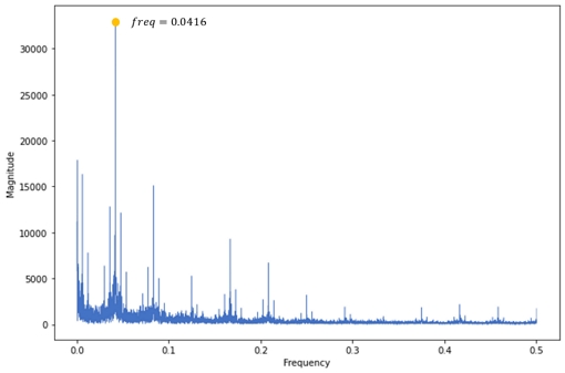
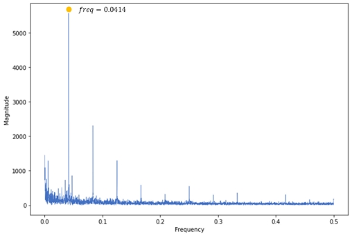
Illustrative Example: To illustrate this methodology, let us consider an example using the Gyeonggi-do and Spain dataset. Fig. 4 and Fig. 5 presents the transformation of the original time series data into its corresponding frequency and magnitude representations. These visualization clearly demonstrates the process of identifying the dominant frequencies within the data. By analyzing the spectral density plot, we can observe the inverse peaks in the frequency domain that correspond to these dominant frequencies. For both the Gyeonggi-do dataset and the additional dataset examined, the estimated 'chronocycle' period c was uniformly determined to be 24 hours.

Fig. 4.

Amplitude spectrum of the Gyeonggi-do dataset

Fig. 5.

Amplitude spectrum of the Spain dataset

Integration into ChronoPatternNet: With the "chronocycle" hyperparameter established, ChronoPatternNet organizes the historical data into structured frames, each encapsulating the identified cyclic nature of electricity usage patterns. This structuring is critical for the subsequent 2D convolutional processing, ensuring that the convolutional layers are attuned to the most significant periodic features in the data, thus enhancing the model’s predictive accuracy.

Ⅳ. Experiments

In our experiment, we evaluated both the parameter count and the predictive efficacy of the out method with TCN, LSTMs, GRUs and ARIMA. The primary goal was to assess the model's performance in accurately forecasting electricity consumption over varying horizons, and its efficiency in both training and inference.

4-1 Dataset

The key statistics of the datasets corpus are summarized in Table 1.

Table 1.

Summary of dataset

Dataset 1: Energy Consumption from Spain (Spain) : The Spain dataset offers hourly energy consumption data, combined with outside temperatures and metadata for 499 customers, available online[37]. Covering a period from January 1 to December 31, 2019, it provides a comprehensive set of 8,760 data points. Our analysis primarily focuses on the total electricity consumption of a particular customer ID, which is representative of typical consumption patterns.

Dataset 2: Gyeonggi-do Building Power Usage (Gyeonggi): The Gyeonggi dataset encompasses hourly records of electricity usage for about 1.9 years, from January 1, 2021, to January 14, 2022. The dataset contains data from around 17,001 commercial buildings in Gyeonggi Province, South Korea, also accessible online[38]. For our research, we specifically concentrate on the building identified by ID 9654, chosen due to its comprehensive and complete data record.

For both datasets, we employed min-max normalization, rescaling features to a [0, 1] range, crucial for maintaining consistency in our analyses. The data was chronologically divided into training (80%), validation (10%), and testing (10%) sets, ensuring the preservation of temporal patterns essential for accurate time series forecasting. This normalization process for a time series data point h_t is mathematically represented as:

$\[ h_{t_{norm}}=\frac{h_t-\text{min}\left(H\right)}{\text{max}\left(H\right)-\text{min}\left(H\right)} \]$

(5)

where h_tnorm denotes the normalized value, and H represents the entire set of historical data points.

4-3 Model Comparison and Analysis

In this section, we compare the performance of the ChronoPatternNet model against several well established models in the field of time series forecasting, such as LSTM, MLP, GRU, TCN, and ARIMA. This comparison is crucial to validate the effectiveness of ChronoPatternNet across various forecasting horizons. The Table 2 and Table 3 summarizes the MSE and MAE values at various forecasting horizons.

Table 2.

Performance on Gyeonggi dataset

Table 3.

Performance on Spain dataset

As illustrated in Table 2, ChronoPatternNet demonstrated better performance than the other models with a margin of (13.42%, 9.07%) for LSTM, (6.63%, 9.73%) for MLP, (14.97%, 11.07%) for GRU, (6.50%, 7.80%) for TCN and (54.92%, 28.01%) for ARIMA. This was especially significant in long-term forecasts (60 to 120 time steps), where ChronoPatternNet's advanced pattern recognition capabilities became most apparent. The consistency in its performance across different forecast ranges accentuates its reliability and accuracy in handling complex time series data.

Similarly, the Spain dataset analysis, as detailed in Table 3, ChronoPatternNet outshone its counterparts with margins of (10.67%, 7.06%) for LSTM, (6.36%, 3.69%) for MLP, (4.14%, 2.77%) for GRU, (12.18%, 6.60%) for TCN, (65.88%, 45.92%) for ARIMA. This performance is a testament to ChronoPatternNet's robustness and adaptability in different temporal contexts, particularly in handling the complexities of longer forecasting horizons.

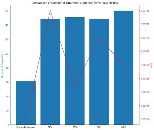
We further compare the model’s parameters in Fig. 6 as well as the error in the experiment when forecasting range is 1 hour. The comparison of model parameters and error rates MSE revealed that ChronoPatternNet, despite having fewer parameters, achieved the lowest error values. This indicates a higher degree of efficiency, where the model delivers optimal performance without the overhead of excessive computational resources.

Fig. 6.

Number of parameters and error comparison

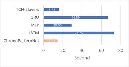
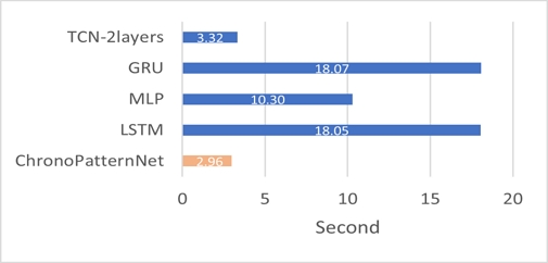
To further emphasize the robustness of our method, we measure the average training and inference time, Fig. 7 and Fig. 8. The average training and inference times were significantly lower for ChronoPatternNet compared to other models. This aspect is particularly crucial in scenarios where realtime data processing and forecasting are required, emphasizing the model's applicability in time sensitive domains.

Fig. 7.

Average training time

Fig. 8

Average inference time

The comprehensive evaluation of ChronoPatternNet reveals its remarkable efficacy and adaptability across varied datasets, highlighting its robustness in different environmental conditions. Its capability for long-term forecasting is noteworthy, demonstrating an advanced algorithmic design adept at handling complex, extended temporal patterns. The model's resilience in managing large errors, a critical feature in real world applications, is evident from its performance in both MSE and MAE error metrics. Additionally, ChronoPatternNet's operational efficiency is marked by its streamlined architecture, leading to lower error rates and reduced training and inference times, making it a highly practical tool for realtime forecasting. Overall, ChronoPatternNet stands out as a versatile, reliable, and efficient solution for a wide range of forecasting challenges.

Ⅴ. Conclusion

ChronoPatternNet, introduced in this study, marks a significant advancement in electricity consumption forecasting, primarily through its innovative approach to temporal pattern recognition. This model excels in identifying repetitive patterns in electricity usage data, thereby enhancing forecasting accuracy significantly. Its design optimizes computational efficiency, making it well suited for realtime forecasting in environments with limited resources. However, its application is predominantly effective in scenarios involving short-term, recurrent data patterns, particularly in household electricity consumption.

The model's current limitations, notably the lack of full automation and challenges in hyperparameter selection, restrict its broader applicability. ChronoPatternNet requires manual hyperparameter tuning, a process that can be cumbersome and inefficient, particularly for data sequences with sparse or extended repetition cycles. Additionally, its design confines its use to univariable datasets, limiting its effectiveness in multivariable time series forecasting.

For future work, enhancing ChronoPatternNet entails focusing on three pivotal areas. Firstly, automated hyperparameter optimization, using advanced techniques like Bayesian optimization or evolutionary algorithms, can automate tuning and optimize performance across varied datasets. Secondly, expansion to multivariable forecasting involves adapting the architecture for multivariable time series, incorporating attention mechanisms or dimensionality reduction, enabling it to forecast scenarios with interrelated variables like industrial power or urban energy management. Lastly, longer-term forecasting capabilities, extending the model's proficiency to longer-term predictions through recurrent neural networks or advanced sequence modeling, is essential. These advancements will broaden ChronoPatternNet's applicability, making it a versatile tool in various sectors, including residential to large-scale industrial applications, and position it as a leading forecasting tool.

Acknowledgments

This work was partly supported by Institute of Information & communications Technology Planning & Evaluation (IITP) grant funded by the Korea government (MSIT) (No. 2021-0-02068, Artificial Intelligence Innovation Hub).

References

• A. Rahmani, M. Khadem, E. Madreseh, H.-A. Aghaei, M. Raei, and M. Karchani, “Descriptive Study of Occupational Accidents and Their Causes among Electricity Distribution Company Workers at an Eight-Year Period in Iran,” Safety and Health at Work, Vol. 4, No. 3, pp. 160-165, September 2013. [https://doi.org/10.1016/j.shaw.2013.07.005]
• D. Xiao, Q. Ma, Y. Xie, Q. Zheng, and Z. Zhang, “A Power-Frequency Electric Field Sensor for Portable Measurement,” Sensors, Vol. 18, No. 4, 1053, March 2018. [https://doi.org/10.3390/s18041053]
• J. L. M. Sabóia, “Autoregressive Integrated Moving Average (ARIMA) Models for Birth Forecasting,” Journal of the American Statistical Association, Vol. 72, No. 358, pp. 264-270, 1977. [https://doi.org/10.1080/01621459.1977.10480989]
• D. J. C. MacKay, Introduction to Gaussian Processes, in Neural Networks and Machine Learning, Berlin, Germany: Springer, ch. 11, pp. 133-165, 1998.
• F. Mahia, A. R. Dey, M. A. Masud, and M. S. Mahmud, “Forecasting Electricity Consumption Using ARIMA Model,” in Proceedings of the International Conference on Sustainable Technologies for Industry 4.0 (STI), Dhaka, Bangladesh, pp. 1-6, December 2019. [https://doi.org/10.1109/STI47673.2019.9068076]
• S. J. E. Parreño, “Forecasting Electricity Consumption in the Philippines Using ARIMA Models,” International Journal of Machine Learning and Computing, Vol. 12, No. 6, pp. 279-285, November 2022. [https://doi.org/10.18178/ijmlc.2022.12.6.1112]
• K. Wen, W. Wu, and X. Wu, “Electricity Demand Forecasting and Risk Management Using Gaussian Process Model with Error Propagation,” Journal of Forecasting, Vol. 42, No. 4, pp. 957-969, July 2023. [https://doi.org/10.1002/for.2925]
• Q. Wen, T. Zhou, C. Zhang, W. Chen, Z. Ma, J. Yan, and L. Sun, “Transformers in Time Series: A Survey,” in Proceedings of the 32nd International Joint Conference on Artificial Intelligence (IJCAI 2023), Macao, pp. 6778-6786, May 2023. [https://doi.org/10.24963/ijcai.2023/759]
• S. Mahjoub, L. Chrifi-Alaoui, B. Marhic, and L. Delahoche, “Predicting Energy Consumption Using LSTM, Multi-Layer GRU and Drop-GRU Neural Networks,” Sensors, Vol. 22, No. 11, 4062, May 2022. [https://doi.org/10.3390/s22114062]
• S. Bai, J. Z. Kolter, and V. Koltun, “An Empirical Evaluation of Generic Convolutional and Recurrent Networks for Sequence Modeling,” arXiv:1803.01271, , April 2018. [https://doi.org/10.48550/arXiv.1803.01271]
• A. Zeng, M. Chen, L. Zhang, and Q. Xu, “Are Transformers Effective for Time Series Forecasting?,” in Proceedings of the 37th AAAI Conference on Artificial Intelligence (AAAI-23), Washington, D.C., pp. 11121-11128, February 2023. [https://doi.org/10.1609/aaai.v37i9.26317]
• R. Shao and X.-J. Bi, “Transformers Meet Small Datasets,” IEEE Access, Vol. 10, pp. 118454-118464, November 2022. [https://doi.org/10.1109/ACCESS.2022.3221138]
• B. Lim and S. Zohren, “Time-Series Forecasting with Deep Learning: A Survey,” Philosophical Transactions of the Royal Society A: Mathematical, Physical and Engineering Sciences, Vol. 379, No. 2194, 20200209, April 2021. [https://doi.org/10.1098/rsta.2020.0209]
• B. Nepal, M. Yamaha, A. Yokoe, and T. Yamaji, “Electricity Load Forecasting Using Clustering and ARIMA Model for Energy Management in Buildings,” Japan Architectural Review, Vol. 3, No. 1, pp. 62-76, January 2020. [https://doi.org/10.1002/2475-8876.12135]
• Y. Chen, P. Xu, Y. Chu, W. Li, Y. Wu, L. Ni, ... and K. Wang, “Short-Term Electrical Load Forecasting Using the Support Vector Regression (SVR) Model to Calculate the Demand Response Baseline for Office Buildings,” Applied Energy, Vol. 195, pp. 659-670, June 2017. [https://doi.org/10.1016/j.apenergy.2017.03.034]
• N. Fumo and M. A. R. Biswas, “Regression Analysis for Prediction of Residential Energy Consumption,” Renewable and Sustainable Energy Reviews, Vol. 47, pp. 332-343, July 2015. [https://doi.org/10.1016/j.rser.2015.03.035]
• J. Zheng, C. Xu, Z. Zhang, and X. Li, “Electric Load Forecasting in Smart Grids Using Long-Short-Term-Memory Based Recurrent Neural Network,” in Proceedings of the 51st Annual Conference on Information Sciences and Systems (CISS), Baltimore: MD, pp. 1-6, March 2017. [https://doi.org/10.1109/CISS.2017.7926112]
• G. Lai, W.-C. Chang, Y. Yang, and H. Liu, “Modeling Long- and Short-Term Temporal Patterns with Deep Neural Networks,” in Proceedings of the 41st International ACM SIGIR Conference on Research & Development in Information Retrieval (SIGIR ’18), Ann Arbor: MI, pp. 95-104, July 2018. [https://doi.org/10.1145/3209978.3210006]
• D. L. Marino, K. Amarasinghe, and M. Manic, “Building Energy Load Forecasting Using Deep Neural Networks,” in Proceedings of the 42nd Annual Conference of the IEEE Industrial Electronics Society (IECON 2016), Florence, Italy, pp. 7046-7051, October 2016. [https://doi.org/10.1109/IECON.2016.7793413]
• D. Li, G. Sun, S. Miao, Y. Gu, Y. Zhang, and S. He, “A Short-Term Electric Load Forecast Method Based on Improved Sequence-to-Sequence GRU with Adaptive Temporal Dependence,” International Journal of Electrical Power and Energy Systems, Vol. 137, 107627, May 2022. [https://doi.org/10.1016/j.ijepes.2021.107627]
• D. Salinas, V. Flunkert, J. Gasthaus, and T. Januschowski, “DeepAR: Probabilistic Forecasting with Autoregressive Recurrent Networks,” International Journal of Forecasting, Vol. 36, No. 3, pp. 1181-1191, July-September 2020. [https://doi.org/10.1016/j.ijforecast.2019.07.001]
• M. Liu, A. Zeng, M. Chen, Z. Xu, Q. Lai, L. Ma, and Q. Xu, “SCINet: Time Series Modeling and Forecasting with Sample Convolution and Interaction,” in Proceedings of the 36th Conference on Neural Information Processing Systems (NeurIPS 2022), New Orleans: LA, pp. 5816-5828, November-December 2022. [https://doi.org/10.48550/arXiv.2106.09305]
• L. H. Anh, G. H. Yu, D. T. Vu, J. S. Kim, J. I. Lee, J. C. Yoon, and J. Y. Kim, “Stride-TCN for Energy Consumption Forecasting and Its Optimization,” Applied Sciences, Vol. 12, No. 19, 9422, September 2022. [https://doi.org/10.3390/app12199422]
• H. Zhou, S. Zhang, J. Peng, S. Zhang, J. Li, H. Xiong, and W. Zhang, “Informer: Beyond Efficient Transformer for Long Sequence Time-Series Forecasting,” in Proceedings of the 35th AAAI Conference on Artificial Intelligence, Online, pp. 11106-11115, February 2021. [https://doi.org/10.48550/arXiv.2012.07436]
• T. Zhou, Z. Ma, Q. Wen, X. Wang, L. Sun, and R. Jin, “FEDformer: Frequency Enhanced Decomposed Transformer for Long-Term Series Forecasting,” in Proceedings of the 39th International Conference on Machine Learning, Baltimore: MD, pp. 27268-27286, July 2022.
• H. Wu, J. Xu, J. Wang, and M. Long, “Autoformer: Decomposition Transformers with Auto-Correlation for Long-Term Series Forecasting,” in Proceedings of the 35th Conference on Neural Information Processing Systems (NeurIPS 2021), Online, pp. 22419-22430, December 2021. [https://doi.org/10.48550/arXiv.2106.13008]
• A. Das, W. Kong, A. Leach, S. Mathur, R. Sen, and R. Yu, “Long-Term Forecasting with TiDE: Time-Series Dense Encoder,” arXiv:2304.08424v4, , December 2023. [https://doi.org/10.48550/arXiv.2304.08424]
• A. Garza and M. Mergenthaler-Canseco, “TimeGPT-1,” arXiv:2310.03589, , October 2023. [https://doi.org/10.48550/arXiv.2310.03589]
• A. Gu, K. Goel, and C. Ré, “Efficiently Modeling Long Sequences with Structured State Spaces,” arXiv:2111.00396v3, , August 2022. [https://doi.org/10.48550/arXiv.2111.00396]
• A. Gu, I. Johnson, A. Timalsina, A. Rudra, and C. Ré, “How to Train Your Hippo: State Space Models with Generalized Orthogonal Basis Projections,” arXiv:2206.12037v2, , August 2022. [https://doi.org/10.48550/arXiv.2206.12037]
• S. S. Rangapuram, M. Seeger, J. Gasthaus, L. Stella, Y. Wang, and T. Januschowski, “Deep State Space Models for Time Series Forecasting,” in Proceedings of the 32nd Conference on Neural Information Processing Systems (NeurIPS 2018), Montréal, Canada, pp. 7796-7805, December 2018.
• R. Sen, H.-F. Yu, and I. Dhillon, “Think Globally, Act Locally: A Deep Neural Network Approach to High-Dimensional Time Series Forecasting,” in Proceedings of the 33rd Conference on Neural Information Processing Systems (NeurIPS 2019), Vancouver, Canada, pp. 4837-4846, December 2019. [https://doi.org/10.48550/arXiv.1905.03806]
• W. Luo, Y. Li, R. Urtasun, and R. Zemel, “Understanding the Effective Receptive Field in Deep Convolutional Neural Networks,” in Proceedings of the 30th Conference on Neural Information Processing Systems (NIPS 2016), Barcelona, Spain, pp. 4905-4913, December 2016. [https://doi.org/10.48550/arXiv.1701.04128]
• Z. Liu, H. Mao, C.-Y. Wu, C. Feichtenhofer, T. Darrell, and S. Xie, “A ConvNet for the 2020s,” in Proceedings of IEEE/CVF Conference on Computer Vision and Pattern Recognition (CVPR), New Orleans: LA, pp. 11966-11976, June 2022. [https://doi.org/10.1109/CVPR52688.2022.01167]
• H. Musbah, M. El-Hawary, and H. Aly, “Identifying Seasonality in Time Series by Applying Fast Fourier Transform,” in Proceedings of 2019 IEEE Electrical Power and Energy Conference (EPEC), Montréal, Canada, pp. 1-4, October 2019. [https://doi.org/10.1109/EPEC47565.2019.9074776]
• F. J. Galán-Sales, P. Reina-Jiménez, M. Carranza-García, and J. M. Luna-Romera, “An Approach to Enhance Time Series Forecasting by Fast Fourier Transform,” in Proceedings of the 18th International Conference on Soft Computing Models in Industrial and Environmental Applications (SOCO 2023), Salamanca, Spain, pp. 259-268, September 2023. [https://doi.org/10.1007/978-3-031-42529-5_25]
• O. Mey, A. Schneider, O. Enge-Rosenblatt, Y. Bravo, and P. Stenzel, “Prediction of Energy Consumption for Variable Customer Portfolios Including Aleatoric Uncertainty Estimation,” in Proceedings of the 10th International Conference on Power Science and Engineering (ICPSE), Istanbul, Turkey, pp. 61-71, October 2021. [https://doi.org/10.1109/ICPSE53473.2021.9656857]
• L. H. Anh, G.-H. Yu, D. T. Vu, H.-G. Kim, and J.-Y. Kim, “DelayNet: Enhancing Temporal Feature Extraction for Electronic Consumption Forecasting with Delayed Dilated Convolution,” Energies, Vol. 16, No. 22, 7662, November 2023. [https://doi.org/10.3390/en16227662]